“Combining datasets”

“Combining datasets”
dplyr?join - see different types of joining for dplyrinner_join(x, y) - only rows that match for x and y are keptfull_join(x, y) - all rows of x and y are keptleft_join(x, y) - all rows of x are kept even if not merged with yright_join(x, y) - all rows of y are kept even if not merged with xanti_join(x, y) - all rows from x not in y keeping just columns from x.data_As
# A tibble: 2 × 3 State June_vacc_rate May_vacc_rate <chr> <dbl> <dbl> 1 Alabama 0.516 0.514 2 Alaska 0.627 0.626
data_cold
# A tibble: 3 × 2 State April_vacc_rate <chr> <dbl> 1 Maine 0.795 2 Alaska 0.623 3 Vermont 0.82
https://github.com/gadenbuie/tidyexplain/blob/main/images/inner-join.gif


lj <- inner_join(data_As, data_cold)
Joining with `by = join_by(State)`
lj
# A tibble: 1 × 4 State June_vacc_rate May_vacc_rate April_vacc_rate <chr> <dbl> <dbl> <dbl> 1 Alaska 0.627 0.626 0.623
https://raw.githubusercontent.com/gadenbuie/tidyexplain/main/images/left-join.gif


lj <- left_join(data_As, data_cold)
Joining with `by = join_by(State)`
lj
# A tibble: 2 × 4 State June_vacc_rate May_vacc_rate April_vacc_rate <chr> <dbl> <dbl> <dbl> 1 Alabama 0.516 0.514 NA 2 Alaska 0.627 0.626 0.623
tidylog package to log outputsNumbers in parentheses indicate that these rows are not included in the result.
# install.packages("tidylog")
library(tidylog)
left_join(data_As, data_cold)
Joining with `by = join_by(State)` left_join: added one column (April_vacc_rate) > rows only in data_As 1 > rows only in data_cold (2) > matched rows 1 > === > rows total 2
# A tibble: 2 × 4 State June_vacc_rate May_vacc_rate April_vacc_rate <chr> <dbl> <dbl> <dbl> 1 Alabama 0.516 0.514 NA 2 Alaska 0.627 0.626 0.623
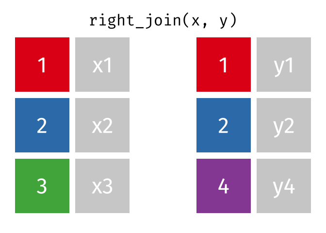
https://raw.githubusercontent.com/gadenbuie/tidyexplain/main/images/right-join.gif


rj <- right_join(data_As, data_cold)
Joining with `by = join_by(State)` right_join: added one column (April_vacc_rate) > rows only in data_As (1) > rows only in data_cold 2 > matched rows 1 > === > rows total 3
rj
# A tibble: 3 × 4 State June_vacc_rate May_vacc_rate April_vacc_rate <chr> <dbl> <dbl> <dbl> 1 Alaska 0.627 0.626 0.623 2 Maine NA NA 0.795 3 Vermont NA NA 0.82
lj2 <- left_join(data_cold, data_As)
Joining with `by = join_by(State)` left_join: added 2 columns (June_vacc_rate, May_vacc_rate) > rows only in data_cold 2 > rows only in data_As (1) > matched rows 1 > === > rows total 3
lj2
# A tibble: 3 × 4 State April_vacc_rate June_vacc_rate May_vacc_rate <chr> <dbl> <dbl> <dbl> 1 Maine 0.795 NA NA 2 Alaska 0.623 0.627 0.626 3 Vermont 0.82 NA NA
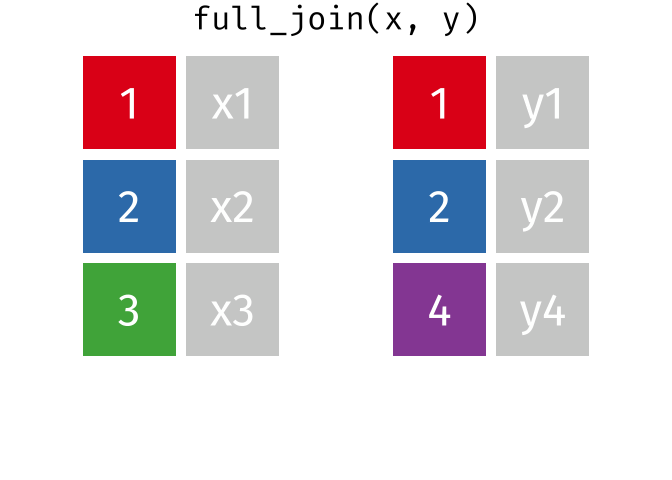
https://raw.githubusercontent.com/gadenbuie/tidyexplain/main/images/full-join.gif


fj <- full_join(data_As, data_cold)
Joining with `by = join_by(State)` full_join: added one column (April_vacc_rate) > rows only in data_As 1 > rows only in data_cold 2 > matched rows 1 > === > rows total 4
fj
# A tibble: 4 × 4 State June_vacc_rate May_vacc_rate April_vacc_rate <chr> <dbl> <dbl> <dbl> 1 Alabama 0.516 0.514 NA 2 Alaska 0.627 0.626 0.623 3 Maine NA NA 0.795 4 Vermont NA NA 0.82
includes duplicates”https://github.com/gadenbuie/tidyexplain/blob/main/images/left-join-extra.gif

tidylogunloadNamespace("tidylog")
Why use join functions?
A. Combine different data sources
B. Connect Rmd to other files
C. Using one data source is too easy and we want our analysis ~ fancy ~
by argumentBy default joins use the intersection of column names. If by is specified, it uses that.
full_join(data_As, data_cold, by = "State")
# A tibble: 4 × 4 State June_vacc_rate May_vacc_rate April_vacc_rate <chr> <dbl> <dbl> <dbl> 1 Alabama 0.516 0.514 NA 2 Alaska 0.627 0.626 0.623 3 Maine NA NA 0.795 4 Vermont NA NA 0.82
by argumentYou can join based on multiple columns by using something like by = c(col1, col2).
If the datasets have two different names for the same data, use:
full_join(x, y, by = c("a" = "b"))
setdiff” (base)We might want to determine what indexes ARE in the first dataset that AREN’T in the second:
data_As
# A tibble: 2 × 3 State June_vacc_rate May_vacc_rate <chr> <dbl> <dbl> 1 Alabama 0.516 0.514 2 Alaska 0.627 0.626
data_cold
# A tibble: 3 × 2 State April_vacc_rate <chr> <dbl> 1 Maine 0.795 2 Alaska 0.623 3 Vermont 0.82
setdiff” (base)Use setdiff to determine what indexes ARE in the first dataset that AREN’T in the second:
A_states <- data_As %>% pull(State) cold_states <- data_cold %>% pull(State)
setdiff(A_states, cold_states)
[1] "Alabama"
setdiff(cold_states, A_states)
[1] "Maine" "Vermont"
bind_rows() (dplyr)Rows are stacked on top of each other. Works like rbind() from base R, but is “smarter” and looks for matching column names.
rbind(data_As, data_cold)
Error in rbind(deparse.level, ...): numbers of columns of arguments do not match
bind_rows(data_As, data_cold)
# A tibble: 5 × 4 State June_vacc_rate May_vacc_rate April_vacc_rate <chr> <dbl> <dbl> <dbl> 1 Alabama 0.516 0.514 NA 2 Alaska 0.627 0.626 NA 3 Maine NA NA 0.795 4 Alaska NA NA 0.623 5 Vermont NA NA 0.82
full_join(data_As, data_cold)
Joining with `by = join_by(State)`
# A tibble: 4 × 4 State June_vacc_rate May_vacc_rate April_vacc_rate <chr> <dbl> <dbl> <dbl> 1 Alabama 0.516 0.514 NA 2 Alaska 0.627 0.626 0.623 3 Maine NA NA 0.795 4 Vermont NA NA 0.82
anti_join (dplyr)
anti_join()https://raw.githubusercontent.com/gadenbuie/tidyexplain/main/images/anti-join.gif

anti_join (dplyr)anti_join(data_As, data_cold)
Joining with `by = join_by(State)`
# A tibble: 1 × 3 State June_vacc_rate May_vacc_rate <chr> <dbl> <dbl> 1 Alabama 0.516 0.514
anti_join (dplyr)anti_join(data_cold, data_As)
Joining with `by = join_by(State)`
# A tibble: 2 × 2 State April_vacc_rate <chr> <dbl> 1 Maine 0.795 2 Vermont 0.82
by = c("a" = "b") if they differinner_join(x, y) - only rows that match for x and y are keptfull_join(x, y) - all rows of x and y are keptleft_join(x, y) - all rows of x are kept even if not merged with yright_join(x, y) - all rows of y are kept even if not merged with xtidylog package for a detailed summarysetdiff(x, y) shows what in x is missing from ybind_rows(x, y) appends datasetshttps://sisbid.github.io/Data-Wrangling/12_Data_Merging/lab/merging-lab.Rmd
There are lots of options for more complicated merges. Check out the documentation if you have a special use case:
cross_join (dplyr)Cross joins match each row in x to every row in y, resulting in a data frame with nrow(x) * nrow(y) rows.
cross_join(data_As, data_cold)
# A tibble: 6 × 5 State.x June_vacc_rate May_vacc_rate State.y April_vacc_rate <chr> <dbl> <dbl> <chr> <dbl> 1 Alabama 0.516 0.514 Maine 0.795 2 Alabama 0.516 0.514 Alaska 0.623 3 Alabama 0.516 0.514 Vermont 0.82 4 Alaska 0.627 0.626 Maine 0.795 5 Alaska 0.627 0.626 Alaska 0.623 6 Alaska 0.627 0.626 Vermont 0.82
nest_join (dplyr)A nest join leaves x almost unchanged, except that it adds a new column for the y dataset. Matched values are stored inside the “cell” as a tibble.
nj <- nest_join(data_As, data_cold)
Joining with `by = join_by(State)`
nj
# A tibble: 2 × 4 State June_vacc_rate May_vacc_rate data_cold <chr> <dbl> <dbl> <list> 1 Alabama 0.516 0.514 <tibble [0 × 1]> 2 Alaska 0.627 0.626 <tibble [1 × 1]>
nest_join (dplyr)nj %>% pull(data_cold)
[[1]]
# A tibble: 0 × 1
# ℹ 1 variable: April_vacc_rate <dbl>
[[2]]
# A tibble: 1 × 1
April_vacc_rate
<dbl>
1 0.623
data_As <- tibble(State = c("Alabama", "Alaska", "Alaska"),
state_bird = c("wild turkey", "willow ptarmigan", "puffin"))
data_cold <- tibble(State = c("Maine", "Alaska", "Alaska"),
vacc_rate = c("32.4%", "41.7%", "46.2%"),
month = c("April", "April", "May"))
full_join(data_As, data_cold)
Joining with `by = join_by(State)`
Warning in full_join(data_As, data_cold): Detected an unexpected many-to-many relationship between `x` and `y`. ℹ Row 2 of `x` matches multiple rows in `y`. ℹ Row 2 of `y` matches multiple rows in `x`. ℹ If a many-to-many relationship is expected, set `relationship = "many-to-many"` to silence this warning.
# A tibble: 6 × 4 State state_bird vacc_rate month <chr> <chr> <chr> <chr> 1 Alabama wild turkey <NA> <NA> 2 Alaska willow ptarmigan 41.7% April 3 Alaska willow ptarmigan 46.2% May 4 Alaska puffin 41.7% April 5 Alaska puffin 46.2% May 6 Maine <NA> 32.4% April