“R, at its heart, is a functional programming (FP) language. This means that it provides many tools for the creation and manipulation of functions.” - Hadley Wickham
Don’t need to write for-loops! - check this video.
“R, at its heart, is a functional programming (FP) language. This means that it provides many tools for the creation and manipulation of functions.” - Hadley Wickham
Don’t need to write for-loops! - check this video.
Allows you to flexibly iterate functions to multiple elements of a data object!
Useful when you want to apply a function to:
* lots of columns in a tibble
* multiple tibbles
* multiple data files
* or perform fancy functions with vectors (or tibble columns)
apply functionsWorks really simply for all columns.
sapply(mtcars, FUN = round)
##       mpg cyl disp  hp drat wt qsec vs am gear carb
##  [1,]  21   6  160 110    4  3   16  0  1    4    4
##  [2,]  21   6  160 110    4  3   17  0  1    4    4
##  [3,]  23   4  108  93    4  2   19  1  1    4    1
##  [4,]  21   6  258 110    3  3   19  1  0    3    1
##  [5,]  19   8  360 175    3  3   17  0  0    3    2
##  [6,]  18   6  225 105    3  3   20  1  0    3    1
##  [7,]  14   8  360 245    3  4   16  0  0    3    4
##  [8,]  24   4  147  62    4  3   20  1  0    4    2
##  [9,]  23   4  141  95    4  3   23  1  0    4    2
## [10,]  19   6  168 123    4  3   18  1  0    4    4
## [11,]  18   6  168 123    4  3   19  1  0    4    4
## [12,]  16   8  276 180    3  4   17  0  0    3    3
## [13,]  17   8  276 180    3  4   18  0  0    3    3
## [14,]  15   8  276 180    3  4   18  0  0    3    3
## [15,]  10   8  472 205    3  5   18  0  0    3    4
## [16,]  10   8  460 215    3  5   18  0  0    3    4
## [17,]  15   8  440 230    3  5   17  0  0    3    4
## [18,]  32   4   79  66    4  2   19  1  1    4    1
## [19,]  30   4   76  52    5  2   19  1  1    4    2
## [20,]  34   4   71  65    4  2   20  1  1    4    1
## [21,]  22   4  120  97    4  2   20  1  0    3    1
## [22,]  16   8  318 150    3  4   17  0  0    3    2
## [23,]  15   8  304 150    3  3   17  0  0    3    2
## [24,]  13   8  350 245    4  4   15  0  0    3    4
## [25,]  19   8  400 175    3  4   17  0  0    3    2
## [26,]  27   4   79  66    4  2   19  1  1    4    1
## [27,]  26   4  120  91    4  2   17  0  1    5    2
## [28,]  30   4   95 113    4  2   17  1  1    5    2
## [29,]  16   8  351 264    4  3   14  0  1    5    4
## [30,]  20   6  145 175    4  3   16  0  1    5    6
## [31,]  15   8  301 335    4  4   15  0  1    5    8
## [32,]  21   4  121 109    4  3   19  1  1    4    2
apply functions specific columnsHarder to use for specific columns.
rounded_mtcars <- mtcars %>% select(disp, drat, wt, qsec) %>%
sapply(FUN = round)
bind_cols(rounded_mtcars, select(mtcars, -c(disp, drat, wt, qsec)))
##                     disp drat wt qsec  mpg cyl  hp vs am gear carb
## Mazda RX4            160    4  3   16 21.0   6 110  0  1    4    4
## Mazda RX4 Wag        160    4  3   17 21.0   6 110  0  1    4    4
## Datsun 710           108    4  2   19 22.8   4  93  1  1    4    1
## Hornet 4 Drive       258    3  3   19 21.4   6 110  1  0    3    1
## Hornet Sportabout    360    3  3   17 18.7   8 175  0  0    3    2
## Valiant              225    3  3   20 18.1   6 105  1  0    3    1
## Duster 360           360    3  4   16 14.3   8 245  0  0    3    4
## Merc 240D            147    4  3   20 24.4   4  62  1  0    4    2
## Merc 230             141    4  3   23 22.8   4  95  1  0    4    2
## Merc 280             168    4  3   18 19.2   6 123  1  0    4    4
## Merc 280C            168    4  3   19 17.8   6 123  1  0    4    4
## Merc 450SE           276    3  4   17 16.4   8 180  0  0    3    3
## Merc 450SL           276    3  4   18 17.3   8 180  0  0    3    3
## Merc 450SLC          276    3  4   18 15.2   8 180  0  0    3    3
## Cadillac Fleetwood   472    3  5   18 10.4   8 205  0  0    3    4
## Lincoln Continental  460    3  5   18 10.4   8 215  0  0    3    4
## Chrysler Imperial    440    3  5   17 14.7   8 230  0  0    3    4
## Fiat 128              79    4  2   19 32.4   4  66  1  1    4    1
## Honda Civic           76    5  2   19 30.4   4  52  1  1    4    2
## Toyota Corolla        71    4  2   20 33.9   4  65  1  1    4    1
## Toyota Corona        120    4  2   20 21.5   4  97  1  0    3    1
## Dodge Challenger     318    3  4   17 15.5   8 150  0  0    3    2
## AMC Javelin          304    3  3   17 15.2   8 150  0  0    3    2
## Camaro Z28           350    4  4   15 13.3   8 245  0  0    3    4
## Pontiac Firebird     400    3  4   17 19.2   8 175  0  0    3    2
## Fiat X1-9             79    4  2   19 27.3   4  66  1  1    4    1
## Porsche 914-2        120    4  2   17 26.0   4  91  0  1    5    2
## Lotus Europa          95    4  2   17 30.4   4 113  1  1    5    2
## Ford Pantera L       351    4  3   14 15.8   8 264  0  1    5    4
## Ferrari Dino         145    4  3   16 19.7   6 175  0  1    5    6
## Maserati Bora        301    4  4   15 15.0   8 335  0  1    5    8
## Volvo 142E           121    4  3   19 21.4   4 109  1  1    4    2
across multiple columnsSay we wanted to round multiple columns of the mtcars data. We could do so one column at a time, or we could use the across function from the dplyr package. Needs to be used within other dplyr functions such as mutate.
mutate(across(which_columns, which function or operation))
head(mtcars, 2)
##               mpg cyl disp  hp drat    wt  qsec vs am gear carb
## Mazda RX4      21   6  160 110  3.9 2.620 16.46  0  1    4    4
## Mazda RX4 Wag  21   6  160 110  3.9 2.875 17.02  0  1    4    4
mtcars %>%
  mutate(across(.cols = c(disp, drat, wt, qsec), round)) %>%
  head(2)
##               mpg cyl disp  hp drat wt qsec vs am gear carb
## Mazda RX4      21   6  160 110    4  3   16  0  1    4    4
## Mazda RX4 Wag  21   6  160 110    4  3   17  0  1    4    4
If you see ~ .x or . this means we are passing x to a function.
See purrr-shortcuts See here for info about the difference between them.
For example - this is not necessary but you could use it here:
mtcars %>%
  mutate(across(.cols = c(disp, drat, wt, qsec), ~ round(.x))) %>%
  head(2)
##               mpg cyl disp  hp drat wt qsec vs am gear carb
## Mazda RX4      21   6  160 110    4  3   16  0  1    4    4
## Mazda RX4 Wag  21   6  160 110    4  3   17  0  1    4    4
mtcars %>%
  mutate(across(.cols = c(disp, drat, wt, qsec), ~ round(.))) %>%
  head(2)
##               mpg cyl disp  hp drat wt qsec vs am gear carb
## Mazda RX4      21   6  160 110    4  3   16  0  1    4    4
## Mazda RX4 Wag  21   6  160 110    4  3   17  0  1    4    4
across with argumentsIf you wish to also pass arguments to the function that you are applying to the various columns, then you need to use the ~ and .x (or .) as a place holder for what you the values you will be passing into the function.
mtcars %>%
  mutate(across(.cols = c(disp, drat, wt, qsec), ~ round(.x, digits = 1))) %>%
  head(n = 2)
##               mpg cyl disp  hp drat  wt qsec vs am gear carb
## Mazda RX4      21   6  160 110  3.9 2.6 16.5  0  1    4    4
## Mazda RX4 Wag  21   6  160 110  3.9 2.9 17.0  0  1    4    4
mtcars %>%
  mutate(across(.cols = c(disp, drat, wt, qsec), ~ round(., digits = 1))) %>%
  head(n = 2)
##               mpg cyl disp  hp drat  wt qsec vs am gear carb
## Mazda RX4      21   6  160 110  3.9 2.6 16.5  0  1    4    4
## Mazda RX4 Wag  21   6  160 110  3.9 2.9 17.0  0  1    4    4
Dilemma: Seems a bit repetitive!
mtcars %>%
  filter(cyl > 3 & cyl < 8,
         gear > 3 & gear < 8,
         carb > 3 & carb < 8)
##                mpg cyl  disp  hp drat    wt  qsec vs am gear carb
## Mazda RX4     21.0   6 160.0 110 3.90 2.620 16.46  0  1    4    4
## Mazda RX4 Wag 21.0   6 160.0 110 3.90 2.875 17.02  0  1    4    4
## Merc 280      19.2   6 167.6 123 3.92 3.440 18.30  1  0    4    4
## Merc 280C     17.8   6 167.6 123 3.92 3.440 18.90  1  0    4    4
## Ferrari Dino  19.7   6 145.0 175 3.62 2.770 15.50  0  1    5    6
if_all(): helps us filter on multiple similar conditions simultaneously!
mtcars %>%
   filter(if_all(c(cyl, gear, carb), ~.x > 3 & .x < 8))
##                mpg cyl  disp  hp drat    wt  qsec vs am gear carb
## Mazda RX4     21.0   6 160.0 110 3.90 2.620 16.46  0  1    4    4
## Mazda RX4 Wag 21.0   6 160.0 110 3.90 2.875 17.02  0  1    4    4
## Merc 280      19.2   6 167.6 123 3.92 3.440 18.30  1  0    4    4
## Merc 280C     17.8   6 167.6 123 3.92 3.440 18.90  1  0    4    4
## Ferrari Dino  19.7   6 145.0 175 3.62 2.770 15.50  0  1    5    6
To create a function we can use the function function and specify what input the function will take and what it will do to it.
my_function <- function(x){x + 1}
my_function
## function(x){x + 1}
## <environment: 0x1040561c8>
my_data  <- c(2,3,4)

my_function(x = my_data)
## [1] 3 4 5
my_function(my_data)
## [1] 3 4 5
Alternatively we can use \(x). See this link about function shortcuts.
my_function <- \(x){x + 1}
my_function
## \(x){x + 1}
## <environment: 0x1040561c8>
my_function(x = my_data)
## [1] 3 4 5
purrr is also a super helpful package!“Designed to make your functions purrr.”
dplyr is designed for data frames purrr is designed for vectors
The purrr package can be very helpful!
purrr main functionsmap and map_* and modify
- applies function to each element of an vector or object (map returns a list, modify returns the same object type) - map_df will output a dataframe
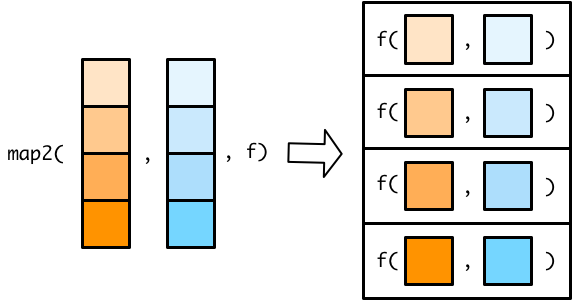
map2 and map2*
- applies function to each element of two vectors or objects
pmap and pmap_* - applies function to each element of 3+ vector or objects (requires a list for input)
the _* options specify the type of data output
map()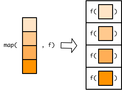 [source]
map_df() amd modify()my_tibble <- tibble(values = c(1.2, 2.3, 3.5, 4.6)) map_df(my_tibble, round)
## # A tibble: 4 × 1
##   values
##    <dbl>
## 1      1
## 2      2
## 3      4
## 4      5
modify(my_tibble, round)
## # A tibble: 4 × 1
##   values
##    <dbl>
## 1      1
## 2      2
## 3      4
## 4      5
But across keeps rownames.
mtcars %>%
  modify(format, digits = 1) %>%
  head(n = 2)
##   mpg cyl disp  hp drat wt qsec vs am gear carb
## 1  21   6  160 110    4  3   16  0  1    4    4
## 2  21   6  160 110    4  3   17  0  1    4    4
mtcars %>%
  mutate(across(.cols = everything(), ~ format(.x, digits = 1))) %>%
  head(n = 2)
##               mpg cyl disp  hp drat wt qsec vs am gear carb
## Mazda RX4      21   6  160 110    4  3   16  0  1    4    4
## Mazda RX4 Wag  21   6  160 110    4  3   17  0  1    4    4
purrr apply function to some columns like acrossUsing modify_if() (or map_if()), we can specify what columns to modify
head(as_tibble(iris), 3)
## # A tibble: 3 × 5
##   Sepal.Length Sepal.Width Petal.Length Petal.Width Species
##          <dbl>       <dbl>        <dbl>       <dbl> <fct>
## 1          5.1         3.5          1.4         0.2 setosa
## 2          4.9         3            1.4         0.2 setosa
## 3          4.7         3.2          1.3         0.2 setosa
as_tibble(iris) %>%
  modify_if(is.numeric, as.character) %>%
  head(3)
## # A tibble: 3 × 5
##   Sepal.Length Sepal.Width Petal.Length Petal.Width Species
##   <chr>        <chr>       <chr>        <chr>       <fct>
## 1 5.1          3.5         1.4          0.2         setosa
## 2 4.9          3           1.4          0.2         setosa
## 3 4.7          3.2         1.3          0.2         setosa
mylist <- list(
  letters = c("A", "b", "c"),
  numbers = 1:3,
  matrix(1:25, ncol = 5),
  matrix(1:25, ncol = 5)
)
head(mylist)
## $letters
## [1] "A" "b" "c"
##
## $numbers
## [1] 1 2 3
##
## [[3]]
##      [,1] [,2] [,3] [,4] [,5]
## [1,]    1    6   11   16   21
## [2,]    2    7   12   17   22
## [3,]    3    8   13   18   23
## [4,]    4    9   14   19   24
## [5,]    5   10   15   20   25
##
## [[4]]
##      [,1] [,2] [,3] [,4] [,5]
## [1,]    1    6   11   16   21
## [2,]    2    7   12   17   22
## [3,]    3    8   13   18   23
## [4,]    4    9   14   19   24
## [5,]    5   10   15   20   25
mylist[1] # returns a list
## $letters
## [1] "A" "b" "c"
mylist["letters"] # returns a list
## $letters
## [1] "A" "b" "c"
mylist[[1]] # returns the vector 'letters'
## [1] "A" "b" "c"
mylist$letters # returns vector
## [1] "A" "b" "c"
mylist[["letters"]] # returns the vector 'letters'
## [1] "A" "b" "c"
You can also select multiple lists with the single brackets.
mylist[1:2] # returns a list
## $letters
## [1] "A" "b" "c"
##
## $numbers
## [1] 1 2 3
split() a datasetWe can create a list by splitting up a dataframe. We will use mtcars.
head(mtcars)
##                    mpg cyl disp  hp drat    wt  qsec vs am gear carb
## Mazda RX4         21.0   6  160 110 3.90 2.620 16.46  0  1    4    4
## Mazda RX4 Wag     21.0   6  160 110 3.90 2.875 17.02  0  1    4    4
## Datsun 710        22.8   4  108  93 3.85 2.320 18.61  1  1    4    1
## Hornet 4 Drive    21.4   6  258 110 3.08 3.215 19.44  1  0    3    1
## Hornet Sportabout 18.7   8  360 175 3.15 3.440 17.02  0  0    3    2
## Valiant           18.1   6  225 105 2.76 3.460 20.22  1  0    3    1
split() the dataset by cylmtcars_split <-mtcars %>% split(.$cyl) str(mtcars_split)
## List of 3
##  $ 4:'data.frame':   11 obs. of  11 variables:
##   ..$ mpg : num [1:11] 22.8 24.4 22.8 32.4 30.4 33.9 21.5 27.3 26 30.4 ...
##   ..$ cyl : num [1:11] 4 4 4 4 4 4 4 4 4 4 ...
##   ..$ disp: num [1:11] 108 146.7 140.8 78.7 75.7 ...
##   ..$ hp  : num [1:11] 93 62 95 66 52 65 97 66 91 113 ...
##   ..$ drat: num [1:11] 3.85 3.69 3.92 4.08 4.93 4.22 3.7 4.08 4.43 3.77 ...
##   ..$ wt  : num [1:11] 2.32 3.19 3.15 2.2 1.61 ...
##   ..$ qsec: num [1:11] 18.6 20 22.9 19.5 18.5 ...
##   ..$ vs  : num [1:11] 1 1 1 1 1 1 1 1 0 1 ...
##   ..$ am  : num [1:11] 1 0 0 1 1 1 0 1 1 1 ...
##   ..$ gear: num [1:11] 4 4 4 4 4 4 3 4 5 5 ...
##   ..$ carb: num [1:11] 1 2 2 1 2 1 1 1 2 2 ...
##  $ 6:'data.frame':   7 obs. of  11 variables:
##   ..$ mpg : num [1:7] 21 21 21.4 18.1 19.2 17.8 19.7
##   ..$ cyl : num [1:7] 6 6 6 6 6 6 6
##   ..$ disp: num [1:7] 160 160 258 225 168 ...
##   ..$ hp  : num [1:7] 110 110 110 105 123 123 175
##   ..$ drat: num [1:7] 3.9 3.9 3.08 2.76 3.92 3.92 3.62
##   ..$ wt  : num [1:7] 2.62 2.88 3.21 3.46 3.44 ...
##   ..$ qsec: num [1:7] 16.5 17 19.4 20.2 18.3 ...
##   ..$ vs  : num [1:7] 0 0 1 1 1 1 0
##   ..$ am  : num [1:7] 1 1 0 0 0 0 1
##   ..$ gear: num [1:7] 4 4 3 3 4 4 5
##   ..$ carb: num [1:7] 4 4 1 1 4 4 6
##  $ 8:'data.frame':   14 obs. of  11 variables:
##   ..$ mpg : num [1:14] 18.7 14.3 16.4 17.3 15.2 10.4 10.4 14.7 15.5 15.2 ...
##   ..$ cyl : num [1:14] 8 8 8 8 8 8 8 8 8 8 ...
##   ..$ disp: num [1:14] 360 360 276 276 276 ...
##   ..$ hp  : num [1:14] 175 245 180 180 180 205 215 230 150 150 ...
##   ..$ drat: num [1:14] 3.15 3.21 3.07 3.07 3.07 2.93 3 3.23 2.76 3.15 ...
##   ..$ wt  : num [1:14] 3.44 3.57 4.07 3.73 3.78 ...
##   ..$ qsec: num [1:14] 17 15.8 17.4 17.6 18 ...
##   ..$ vs  : num [1:14] 0 0 0 0 0 0 0 0 0 0 ...
##   ..$ am  : num [1:14] 0 0 0 0 0 0 0 0 0 0 ...
##   ..$ gear: num [1:14] 3 3 3 3 3 3 3 3 3 3 ...
##   ..$ carb: num [1:14] 2 4 3 3 3 4 4 4 2 2 ...
mtcars %>%
  split(.$cyl) %>% # creates split of data for each unique cyl value
  map(~lm(mpg ~ wt, data = .)) %>% # apply linear model to each
  map(summary) %>%
  map_dbl("r.squared")
##         4         6         8
## 0.5086326 0.4645102 0.4229655
This comes up a lot in data cleaning and also when reading in multiple files!
library(here)
library(readr)
file_list <- list.files(here::here("data/iris/"), pattern = "*.csv")

file_list <- paste0(here::here("data/iris/"), file_list)
file_list
## [1] "/Users/avahoffman/Dropbox/JHSPH/Data-Wrangling_SISBID/data/iris/iris_q1.csv"
## [2] "/Users/avahoffman/Dropbox/JHSPH/Data-Wrangling_SISBID/data/iris/iris_q4.csv"
## [3] "/Users/avahoffman/Dropbox/JHSPH/Data-Wrangling_SISBID/data/iris/iris_q5.csv"
multifile_data <- file_list %>%
  map(read_csv)
multifile_data[[1]]
## # A tibble: 150 × 5
##    Sepal.Length Sepal.Width Petal.Length Petal.Width Species
##           <dbl>       <dbl>        <dbl>       <dbl> <chr>
##  1          5.1         3.5          1.4         0.2 setosa
##  2          4.9         3            1.4         0.2 setosa
##  3          4.7         3.2          1.3         0.2 setosa
##  4          4.6         3.1          1.5         0.2 setosa
##  5          5           3.6          1.4         0.2 setosa
##  6          5.4         3.9          1.7         0.4 setosa
##  7          4.6         3.4          1.4         0.3 setosa
##  8          5           3.4          1.5         0.2 setosa
##  9          4.4         2.9          1.4         0.2 setosa
## 10          4.9         3.1          1.5         0.1 setosa
## # ℹ 140 more rows
multifile_data[[2]]
## # A tibble: 150 × 1
##    `Sepal.Length:Sepal.Width:Petal.Length:Petal.Width:Species`
##    <chr>
##  1 5.1:3.5:1.4:0.2:setosa
##  2 4.9:3:1.4:0.2:setosa
##  3 4.7:3.2:1.3:0.2:setosa
##  4 4.6:3.1:1.5:0.2:setosa
##  5 5:3.6:1.4:0.2:setosa
##  6 5.4:3.9:1.7:0.4:setosa
##  7 4.6:3.4:1.4:0.3:setosa
##  8 5:3.4:1.5:0.2:setosa
##  9 4.4:2.9:1.4:0.2:setosa
## 10 4.9:3.1:1.5:0.1:setosa
## # ℹ 140 more rows
multifile_data[[3]]
## # A tibble: 150 × 5
##    Sepal.Length Sepal.Width Petal.Length Petal.Width Species
##           <dbl>       <dbl>        <dbl>       <dbl> <chr>
##  1       -999           3.5          1.4         0.2 setosa
##  2       -999           3            1.4         0.2 setosa
##  3       -999           3.2          1.3         0.2 setosa
##  4          4.6         3.1          1.5         0.2 setosa
##  5          5           3.6          1.4         0.2 setosa
##  6          5.4         3.9          1.7         0.4 setosa
##  7          4.6         3.4          1.4         0.3 setosa
##  8          5           3.4          1.5         0.2 setosa
##  9          4.4         2.9          1.4         0.2 setosa
## 10          4.9         3.1          1.5         0.1 setosa
## # ℹ 140 more rows
delimiters <- c(",", ":", ",")  # delimiters for each file

# Write our own function to read files with specific delimiters:

read_with_delimiter <- function(file, delimiter) {
  read_delim(file, delim = delimiter)
}

# Map over file_list and delimiters
multifile_data <- map2(file_list, delimiters, read_with_delimiter)
[source]
multifile_data[[1]]
## # A tibble: 150 × 5
##    Sepal.Length Sepal.Width Petal.Length Petal.Width Species
##           <dbl>       <dbl>        <dbl>       <dbl> <chr>
##  1          5.1         3.5          1.4         0.2 setosa
##  2          4.9         3            1.4         0.2 setosa
##  3          4.7         3.2          1.3         0.2 setosa
##  4          4.6         3.1          1.5         0.2 setosa
##  5          5           3.6          1.4         0.2 setosa
##  6          5.4         3.9          1.7         0.4 setosa
##  7          4.6         3.4          1.4         0.3 setosa
##  8          5           3.4          1.5         0.2 setosa
##  9          4.4         2.9          1.4         0.2 setosa
## 10          4.9         3.1          1.5         0.1 setosa
## # ℹ 140 more rows
multifile_data[[2]]
## # A tibble: 150 × 5
##    Sepal.Length Sepal.Width Petal.Length Petal.Width Species
##           <dbl>       <dbl>        <dbl>       <dbl> <chr>
##  1          5.1         3.5          1.4         0.2 setosa
##  2          4.9         3            1.4         0.2 setosa
##  3          4.7         3.2          1.3         0.2 setosa
##  4          4.6         3.1          1.5         0.2 setosa
##  5          5           3.6          1.4         0.2 setosa
##  6          5.4         3.9          1.7         0.4 setosa
##  7          4.6         3.4          1.4         0.3 setosa
##  8          5           3.4          1.5         0.2 setosa
##  9          4.4         2.9          1.4         0.2 setosa
## 10          4.9         3.1          1.5         0.1 setosa
## # ℹ 140 more rows
multifile_data[[3]]
## # A tibble: 150 × 5
##    Sepal.Length Sepal.Width Petal.Length Petal.Width Species
##           <dbl>       <dbl>        <dbl>       <dbl> <chr>
##  1       -999           3.5          1.4         0.2 setosa
##  2       -999           3            1.4         0.2 setosa
##  3       -999           3.2          1.3         0.2 setosa
##  4          4.6         3.1          1.5         0.2 setosa
##  5          5           3.6          1.4         0.2 setosa
##  6          5.4         3.9          1.7         0.4 setosa
##  7          4.6         3.4          1.4         0.3 setosa
##  8          5           3.4          1.5         0.2 setosa
##  9          4.4         2.9          1.4         0.2 setosa
## 10          4.9         3.1          1.5         0.1 setosa
## # ℹ 140 more rows
The bind_rows() function can be great for combining data.
recall that modify keeps the same data type (here, a list). We want a data frame instead.
See https://www.opencasestudies.org/ocs-bp-vaping-case-study for more information!
all_files_data <-
  multifile_data %>%
  map_df(bind_rows, .id = "experiment")

glimpse(all_files_data)
## Rows: 450
## Columns: 6
## $ experiment   <chr> "1", "1", "1", "1", "1", "1", "1", "1", "1", "1", "1", "1…
## $ Sepal.Length <dbl> 5.1, 4.9, 4.7, 4.6, 5.0, 5.4, 4.6, 5.0, 4.4, 4.9, 5.4, 4.…
## $ Sepal.Width  <dbl> 3.5, 3.0, 3.2, 3.1, 3.6, 3.9, 3.4, 3.4, 2.9, 3.1, 3.7, 3.…
## $ Petal.Length <dbl> 1.4, 1.4, 1.3, 1.5, 1.4, 1.7, 1.4, 1.5, 1.4, 1.5, 1.5, 1.…
## $ Petal.Width  <dbl> 0.2, 0.2, 0.2, 0.2, 0.2, 0.4, 0.3, 0.2, 0.2, 0.1, 0.2, 0.…
## $ Species      <chr> "setosa", "setosa", "setosa", "setosa", "setosa", "setosa…
function(x){ } or \(x){ } denotes a function. You also commonly see ~.x inside acrossmap_df and modify apply functions to each element of an object. map returns a list, modify returns the same object type.https://sisbid.github.io/Data-Wrangling/14_Functional_Programming/lab/functional-program-lab.Rmd
?tidyr_tidy_select
mtcars %>%
  mutate(across(.cols = disp:wt, round)) %>%
  head(2)
##               mpg cyl disp  hp drat wt  qsec vs am gear carb
## Mazda RX4      21   6  160 110    4  3 16.46  0  1    4    4
## Mazda RX4 Wag  21   6  160 110    4  3 17.02  0  1    4    4
mtcars %>%
  mutate(across(.cols = everything(), round))%>%
  head(2)
##               mpg cyl disp  hp drat wt qsec vs am gear carb
## Mazda RX4      21   6  160 110    4  3   16  0  1    4    4
## Mazda RX4 Wag  21   6  160 110    4  3   17  0  1    4    4
system.time(iris %>%
              modify_if(is.factor, as.character))
##    user  system elapsed
##   0.000   0.000   0.001
system.time(iris %>%
               mutate(across(.cols = where(is.factor), as.character)))
##    user  system elapsed
##   0.001   0.000   0.001
Looks like it had a different delimiter First, separating by the :.
multifile_data[[2]] <-
  separate(
    multifile_data[[2]],
    col = 1,
    into = colnames(multifile_data[[1]]),
    sep = ":"
  )
## Warning: Expected 5 pieces. Missing pieces filled with `NA` in 150 rows [1, 2,
## 3, 4, 5, 6, 7, 8, 9, 10, 11, 12, 13, 14, 15, 16, 17, 18, 19, 20, ...].
head(multifile_data[[2]], 3)
## # A tibble: 3 × 5
##   Sepal.Length Sepal.Width Petal.Length Petal.Width Species
##   <chr>        <chr>       <chr>        <chr>       <chr>
## 1 5.1          <NA>        <NA>         <NA>        <NA>
## 2 4.9          <NA>        <NA>         <NA>        <NA>
## 3 4.7          <NA>        <NA>         <NA>        <NA>
Second, making sure values are numeric.
multifile_data[[2]] <-
  multifile_data[[2]] %>%
  mutate(across(!Species, as.numeric))

head(multifile_data[[2]], 3)
## # A tibble: 3 × 5
##   Sepal.Length Sepal.Width Petal.Length Petal.Width Species
##          <dbl>       <dbl>        <dbl>       <dbl> <chr>
## 1          5.1          NA           NA          NA <NA>
## 2          4.9          NA           NA          NA <NA>
## 3          4.7          NA           NA          NA <NA>
```