“R, at its heart, is a functional programming (FP) language. This means that it provides many tools for the creation and manipulation of functions. In particular, R has what’s known as first class functions. You can do anything with functions that you can do with vectors: you can assign them to variables, store them in lists, pass them as arguments to other functions, create them inside functions, and even return them as the result of a function.” - Hadley Wickham

Don’t need to write for-loops! - check this video.

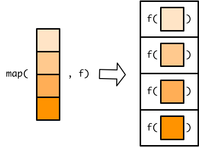
Allows you to flexibly iterate functions to multiple elements of a data object!

Useful when you want to apply a function to:
* lots of columns in a tibble
* multiple tibbles
* multiple data files
* or perform fancy functions with vectors (or tibble columns)

Say we wanted to round multiple columns of the mtcars data. We could do so one column at a time, or we could use the across function from the dplyr package. Needs to be used within other dplyr functions such as mutate.

mutate(across(which_columns, which function or operation))

head(mtcars, 2)

##               mpg cyl disp  hp drat    wt  qsec vs am gear carb
## Mazda RX4      21   6  160 110  3.9 2.620 16.46  0  1    4    4
## Mazda RX4 Wag  21   6  160 110  3.9 2.875 17.02  0  1    4    4

mtcars %>% 
  mutate(across(.cols = c(disp, drat, wt, qsec), round)) %>%
  head(2)

##               mpg cyl disp  hp drat wt qsec vs am gear carb
## Mazda RX4      21   6  160 110    4  3   16  0  1    4    4
## Mazda RX4 Wag  21   6  160 110    4  3   17  0  1    4    4

my_function <- function(x){x + 1} # alt: \(x){x + 1}
my_function

## function(x){x + 1}

my_data  <- c(2,3,4)

my_function(x = my_data)

## [1] 3 4 5

my_function(my_data)

## [1] 3 4 5

?tidyr_tidy_select

mtcars %>% 
  mutate(across(.cols = disp:wt, round)) %>%
  head(2)

##               mpg cyl disp  hp drat wt  qsec vs am gear carb
## Mazda RX4      21   6  160 110    4  3 16.46  0  1    4    4
## Mazda RX4 Wag  21   6  160 110    4  3 17.02  0  1    4    4

mtcars %>% 
  mutate(across(.cols = everything(), round))%>%
  head(2)

##               mpg cyl disp  hp drat wt qsec vs am gear carb
## Mazda RX4      21   6  160 110    4  3   16  0  1    4    4
## Mazda RX4 Wag  21   6  160 110    4  3   17  0  1    4    4

Dilemma: Seems a bit repetitive!

mtcars %>%
  filter(cyl > 3 & cyl < 8,
         gear > 3 & gear < 8,
         carb > 3 & carb < 8)

##                mpg cyl  disp  hp drat    wt  qsec vs am gear carb
## Mazda RX4     21.0   6 160.0 110 3.90 2.620 16.46  0  1    4    4
## Mazda RX4 Wag 21.0   6 160.0 110 3.90 2.875 17.02  0  1    4    4
## Merc 280      19.2   6 167.6 123 3.92 3.440 18.30  1  0    4    4
## Merc 280C     17.8   6 167.6 123 3.92 3.440 18.90  1  0    4    4
## Ferrari Dino  19.7   6 145.0 175 3.62 2.770 15.50  0  1    5    6

if_all(): helps us filter on multiple similar conditions simultaneously!

mtcars %>%
   filter(if_all(c(cyl, gear, carb), ~.x > 3 & .x < 8))

##                mpg cyl  disp  hp drat    wt  qsec vs am gear carb
## Mazda RX4     21.0   6 160.0 110 3.90 2.620 16.46  0  1    4    4
## Mazda RX4 Wag 21.0   6 160.0 110 3.90 2.875 17.02  0  1    4    4
## Merc 280      19.2   6 167.6 123 3.92 3.440 18.30  1  0    4    4
## Merc 280C     17.8   6 167.6 123 3.92 3.440 18.90  1  0    4    4
## Ferrari Dino  19.7   6 145.0 175 3.62 2.770 15.50  0  1    5    6

Work inside other tidyverse functions, like across()

iris %>% filter(Sepal.Length > 2.4 & Sepal.Width > 2.4 &
                Petal.Length > 2.4 & Petal.Width > 2.4)

##   Sepal.Length Sepal.Width Petal.Length Petal.Width   Species
## 1          6.3         3.3          6.0         2.5 virginica
## 2          7.2         3.6          6.1         2.5 virginica
## 3          6.7         3.3          5.7         2.5 virginica

iris %>% filter(if_all(Sepal.Length:Petal.Width, ~ . > 2.4))

##   Sepal.Length Sepal.Width Petal.Length Petal.Width   Species
## 1          6.3         3.3          6.0         2.5 virginica
## 2          7.2         3.6          6.1         2.5 virginica
## 3          6.7         3.3          5.7         2.5 virginica

“Designed to make your functions purrr.”

dplyr is designed for data frames purrr is designed for vectors

The purrr package can be very helpful!

• https://purrr.tidyverse.org/

• https://github.com/rstudio/cheatsheets/raw/master/purrr.pdf

• https://jennybc.github.io/purrr-tutorial/

map and map_* and modify
- applies function to each element of an vector or object (map returns a list, modify returns the same object type)

map2 and map2*
- applies function to each element of two vectors or objects

pmap and pmap_* - applies function to each element of 3+ vector or objects (requires a list for input)

the _* options specify the type of data output

[source]

vect <- c(1.2, 2.3, 3.5, 4.6)
map(vect, round) %>% unlist()

## [1] 1 2 4 5

my_tibble <- tibble(values = c(1.2, 2.3, 3.5, 4.6))
map_df(my_tibble, round)

## # A tibble: 4 × 1
##   values
##    <dbl>
## 1      1
## 2      2
## 3      4
## 4      5

modify(vect, round)

## [1] 1 2 4 5

modify(my_tibble, round)

## # A tibble: 4 × 1
##   values
##    <dbl>
## 1      1
## 2      2
## 3      4
## 4      5

map_df

library(purrr)
head(mtcars, 2)

##               mpg cyl disp  hp drat    wt  qsec vs am gear carb
## Mazda RX4      21   6  160 110  3.9 2.620 16.46  0  1    4    4
## Mazda RX4 Wag  21   6  160 110  3.9 2.875 17.02  0  1    4    4

 mtcars %>% 
   map_df(round) %>%
   head(2)

## # A tibble: 2 × 11
##     mpg   cyl  disp    hp  drat    wt  qsec    vs    am  gear  carb
##   <dbl> <dbl> <dbl> <dbl> <dbl> <dbl> <dbl> <dbl> <dbl> <dbl> <dbl>
## 1    21     6   160   110     4     3    16     0     1     4     4
## 2    21     6   160   110     4     3    17     0     1     4     4

modify

 mtcars %>% 
   modify(round) %>%
   head(2)

##   mpg cyl disp  hp drat wt qsec vs am gear carb
## 1  21   6  160 110    4  3   16  0  1    4    4
## 2  21   6  160 110    4  3   17  0  1    4    4

But across keeps rownames..

mtcars %>% 
  modify(format, digits = 1) %>%
  head(n = 2)

##   mpg cyl disp  hp drat wt qsec vs am gear carb
## 1  21   6  160 110    4  3   16  0  1    4    4
## 2  21   6  160 110    4  3   17  0  1    4    4

mtcars %>% 
  mutate(across(.cols = everything(), ~ format(.x, digits = 1))) %>%
  head(n = 2)

##               mpg cyl disp  hp drat wt qsec vs am gear carb
## Mazda RX4      21   6  160 110    4  3   16  0  1    4    4
## Mazda RX4 Wag  21   6  160 110    4  3   17  0  1    4    4

system.time(iris %>%
              modify_if(is.factor, as.character))

##    user  system elapsed 
##       0       0       0

system.time(iris %>%
               mutate(across(.cols = where(is.factor), as.character)))

##    user  system elapsed 
##   0.001   0.000   0.001

• Lists are the most flexible/“generic” data class in R
• Can be created using list()
• Can hold vectors, strings, matrices, models, list of other lists, lists upon lists!
• Can reference data using $ (if the elements are named), or using [], or [[]]

mylist <- list(
  letters = c("A", "b", "c"),
  numbers = 1:3,
  matrix(1:25, ncol = 5),
  matrix(1:25, ncol = 5)
)

head(mylist)

## $letters
## [1] "A" "b" "c"
## 
## $numbers
## [1] 1 2 3
## 
## [[3]]
##      [,1] [,2] [,3] [,4] [,5]
## [1,]    1    6   11   16   21
## [2,]    2    7   12   17   22
## [3,]    3    8   13   18   23
## [4,]    4    9   14   19   24
## [5,]    5   10   15   20   25
## 
## [[4]]
##      [,1] [,2] [,3] [,4] [,5]
## [1,]    1    6   11   16   21
## [2,]    2    7   12   17   22
## [3,]    3    8   13   18   23
## [4,]    4    9   14   19   24
## [5,]    5   10   15   20   25

mylist[1] # returns a list

## $letters
## [1] "A" "b" "c"

mylist["letters"] # returns a list

## $letters
## [1] "A" "b" "c"

mylist[[1]] # returns the vector 'letters'

## [1] "A" "b" "c"

mylist$letters # returns vector

## [1] "A" "b" "c"

mylist[["letters"]] # returns the vector 'letters'

## [1] "A" "b" "c"

You can also select multiple lists with the single brackets.

mylist[1:2] # returns a list

## $letters
## [1] "A" "b" "c"
## 
## $numbers
## [1] 1 2 3

head(mtcars)

##                    mpg cyl disp  hp drat    wt  qsec vs am gear carb
## Mazda RX4         21.0   6  160 110 3.90 2.620 16.46  0  1    4    4
## Mazda RX4 Wag     21.0   6  160 110 3.90 2.875 17.02  0  1    4    4
## Datsun 710        22.8   4  108  93 3.85 2.320 18.61  1  1    4    1
## Hornet 4 Drive    21.4   6  258 110 3.08 3.215 19.44  1  0    3    1
## Hornet Sportabout 18.7   8  360 175 3.15 3.440 17.02  0  0    3    2
## Valiant           18.1   6  225 105 2.76 3.460 20.22  1  0    3    1

str(mtcars %>% split(.$cyl))

## List of 3
##  $ 4:'data.frame':   11 obs. of  11 variables:
##   ..$ mpg : num [1:11] 22.8 24.4 22.8 32.4 30.4 33.9 21.5 27.3 26 30.4 ...
##   ..$ cyl : num [1:11] 4 4 4 4 4 4 4 4 4 4 ...
##   ..$ disp: num [1:11] 108 146.7 140.8 78.7 75.7 ...
##   ..$ hp  : num [1:11] 93 62 95 66 52 65 97 66 91 113 ...
##   ..$ drat: num [1:11] 3.85 3.69 3.92 4.08 4.93 4.22 3.7 4.08 4.43 3.77 ...
##   ..$ wt  : num [1:11] 2.32 3.19 3.15 2.2 1.61 ...
##   ..$ qsec: num [1:11] 18.6 20 22.9 19.5 18.5 ...
##   ..$ vs  : num [1:11] 1 1 1 1 1 1 1 1 0 1 ...
##   ..$ am  : num [1:11] 1 0 0 1 1 1 0 1 1 1 ...
##   ..$ gear: num [1:11] 4 4 4 4 4 4 3 4 5 5 ...
##   ..$ carb: num [1:11] 1 2 2 1 2 1 1 1 2 2 ...
##  $ 6:'data.frame':   7 obs. of  11 variables:
##   ..$ mpg : num [1:7] 21 21 21.4 18.1 19.2 17.8 19.7
##   ..$ cyl : num [1:7] 6 6 6 6 6 6 6
##   ..$ disp: num [1:7] 160 160 258 225 168 ...
##   ..$ hp  : num [1:7] 110 110 110 105 123 123 175
##   ..$ drat: num [1:7] 3.9 3.9 3.08 2.76 3.92 3.92 3.62
##   ..$ wt  : num [1:7] 2.62 2.88 3.21 3.46 3.44 ...
##   ..$ qsec: num [1:7] 16.5 17 19.4 20.2 18.3 ...
##   ..$ vs  : num [1:7] 0 0 1 1 1 1 0
##   ..$ am  : num [1:7] 1 1 0 0 0 0 1
##   ..$ gear: num [1:7] 4 4 3 3 4 4 5
##   ..$ carb: num [1:7] 4 4 1 1 4 4 6
##  $ 8:'data.frame':   14 obs. of  11 variables:
##   ..$ mpg : num [1:14] 18.7 14.3 16.4 17.3 15.2 10.4 10.4 14.7 15.5 15.2 ...
##   ..$ cyl : num [1:14] 8 8 8 8 8 8 8 8 8 8 ...
##   ..$ disp: num [1:14] 360 360 276 276 276 ...
##   ..$ hp  : num [1:14] 175 245 180 180 180 205 215 230 150 150 ...
##   ..$ drat: num [1:14] 3.15 3.21 3.07 3.07 3.07 2.93 3 3.23 2.76 3.15 ...
##   ..$ wt  : num [1:14] 3.44 3.57 4.07 3.73 3.78 ...
##   ..$ qsec: num [1:14] 17 15.8 17.4 17.6 18 ...
##   ..$ vs  : num [1:14] 0 0 0 0 0 0 0 0 0 0 ...
##   ..$ am  : num [1:14] 0 0 0 0 0 0 0 0 0 0 ...
##   ..$ gear: num [1:14] 3 3 3 3 3 3 3 3 3 3 ...
##   ..$ carb: num [1:14] 2 4 3 3 3 4 4 4 2 2 ...

mtcars %>%
  split(.$cyl) %>% # creates split of data for each unique cyl value
  map(~lm(mpg ~ wt, data = .)) %>% # apply linear model to each
  map(summary) %>%
  map_dbl("r.squared")

##         4         6         8 
## 0.5086326 0.4645102 0.4229655

Second, making sure values are numeric.

multifile_data[[2]] <-
  multifile_data[[2]] %>%
  mutate(across(!Species, as.numeric))

head(multifile_data[[2]], 3)

## # A tibble: 3 × 5
##   Sepal.Length Sepal.Width Petal.Length Petal.Width Species
##          <dbl>       <dbl>        <dbl>       <dbl> <chr>  
## 1          5.1         3.5          1.4         0.2 setosa 
## 2          4.9         3            1.4         0.2 setosa 
## 3          4.7         3.2          1.3         0.2 setosa

• function(x){ } or (x){ } denotes a function. You also commonly see ~.x inside across
• map_df and modify apply functions to each element of an object. map returns a list, modify returns the same object type.
• The purrr package has other useful functional programming features
• lists can be great for storing iterative work.

https://sisbid.github.io/Data-Wrangling/labs/functional-program-lab.Rmd